 Using Acumen Risk to Compare Multiple-Schedule Risk Exposure
Deltek Acumen Risk considers project risks to make a more realistic schedule, but how do you efficiently compare the outcome from two separate Acumen Risk models? Here we take a look at this.
The traditional Critical Path Method (CPM) is deterministic; it computes the schedule completion on an exact day. This date is also the only data point, a single iteration. Deltek Acumen Risk provides at least two advantages over the CPM.
First, Acumen Risk adjusts schedules to make them more realistic. Second, it provides a range of completion dates supplemented by cumulative frequency, i.e., probability. So, where the CPM specifies a completion date, Acumen Risk provides a finish date and certainty in achieving that date.
Acumen Risk uses a Monte Carlo simulation to calculate many iterations or outcomes, each iteration affected by its own set of random numbers. A risk exposure histogram chart reports the outcome from a specified number of iterations.
In addition, Acumen plots the cumulative frequency of occurring dates on this histogram chart, known as the S-curve. This S-curve links schedule completion dates to respective cumulative frequency or confidence levels.
In Acumen Risk, schedulers can compare multiple S-curves of a risk-adjusted schedule. Thus, they can investigate S-curve completion dates and certainty for a schedule risk with varying probability and impact.
Moreover, it can plot S-curves from several risk-adjusted schedules on a graph and measure variance. In this way, a multiple-schedule risk exposure comparison is possible with Acumen Risk software.
This article demonstrates a multiple-schedule risk exposure comparison in Deltek Acumen Risk.
In our demonstration, we will investigate the schedule impact of supplementing a pipe repair project by adding a thrust block. The thrust block keeps the ninety-degree pipe elbows in place whenever the fluid in the associated piping is turned on and off. The pipe repairs and thrust block installation deliverables combine for a repair and improvement project.
We want to know how many days realistically the installation of the thrust block will increase the schedule duration. We must have a completion date that gives us eighty percent certainty we can achieve that date. This would be good to know before we commit to the thrust block installation and a project delivery date.
Figure 1 displays the demonstration pipe repair schedule by itself.
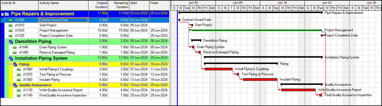 Figure 1
The pipe repair and improvement schedule, including the thrust block, is in Figure 2.
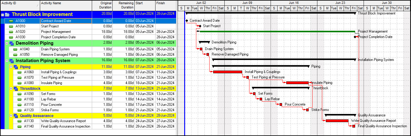 Figure 2
Let us import both schedules into an Acumen Risk workbook. We choose S1 // Projects | Oracle Primavera | Single Project from a P6 XER file, Figure 3.
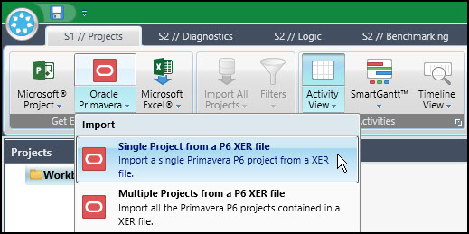 Figure 3
We select the appropriate file in the resulting Open Windows Explorer dialogue. In the Select a Primavera P6 Project dialog, we again select the PIPE REPAIRS schedule. Note that an XER file can have multiple schedules embedded; we only have one. We choose PIPE REPAIRS and OK, Figure 4.
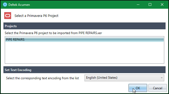 Figure 4
This links the schedule to the Acumen Workbook1, Figure 5.
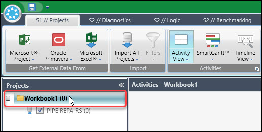 Figure 5
We want to import the second schedule. First, we left-click on the workbook, then again choose S1 // Projects | Oracle Primavera | Single Project from a P6 XER file. In the resulting Select a Primavera P6 Project dialog, we choose the BLOCK schedule, Figure 6.
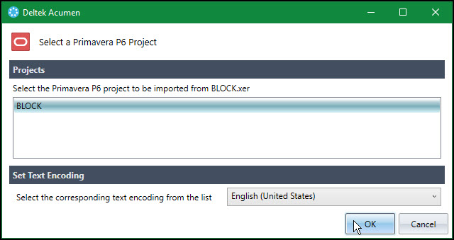 Figure 6
Now, both schedules are linked to the workbook, Figure 7.
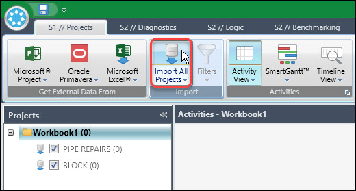 Figure 7
We then finish the import by clicking Import All Projects, Figure 7. The navigator pane with imported projects appears in Figure 8.
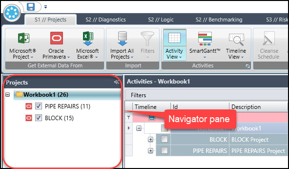 Figure 8
We want to perform a risk analysis but must perform diagnostic analyses to confirm quality schedules before continuing with risk modeling. Proceed and click S2 // Diagnostics, confirm the Schedule Quality is the active metric group, and click Fuse to analyze the quality of the schedules. The output of the Schedule Quality metric group analyses for each schedule is in Figure 9.
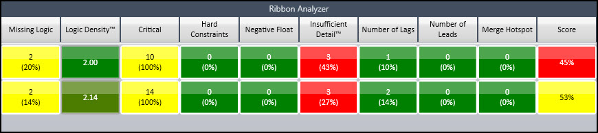 Figure 9
The first row of metric group output in Figure 9 is the PIPE REPAIRS schedule, and the second row is the BLOCK schedule. We review the missing logic metric of the PIPE REPAIRS schedule by clicking its score box, Figure 10.
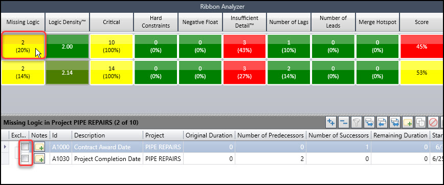 Figure 10
The first and last tasks in the schedule are missing logic, which we would expect. Let us see if our schedule quality Score improves when we remove the Contract Award Date and Project Completion Date from the analysis for the PIPE REPAIRS schedule, Figure 10, and the BLOCK schedule, Figure 11.
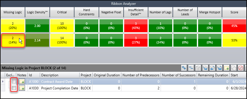 Figure 11
We click to exclude Contract Award Date and Project Completion Date in Figures 10 and 11. We then click the Fuse button to analyze each schedule’s Schedule Quality metric group performance. The Schedule Quality metric group scores improve to 64% and 67% accordingly, Figure 12.
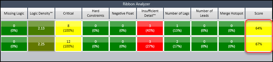 Figure 12
They score better but have room for improvement. Both schedules fail the Insufficient Detail metric, Figure 12. Figure 13 shows that tasks over 10% of the project’s total duration failed the Insufficient Detail metric.
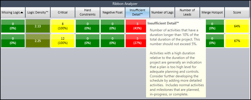 Figure 13
The Insufficient Detail metric flags several tasks due to the short duration of both schedules. Let us make exceptions to these tasks and remove them from the analysis. The resulting Schedule Quality metric analyses appear in Figure 14.
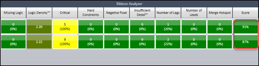 Figure 14
Now, both schedules have a passing score, Figure 14. We are ready to model risk in our schedules. We continue and click S3 // Risk.
The PIPE REPAIRS schedule in the navigator pane defaults as the active, Figure 15.
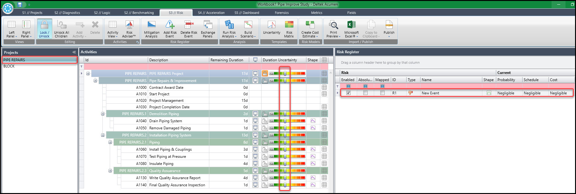 Figure 15
We set the Duration Uncertainty for the entire schedule to Conservative, Figure 16. This indicates that the estimator considers the task duration estimates achievable or better. The Risk Register defaults to a negligible risk event, Figure 15.
The PIPE REPAIR schedule has no risk events, so we leave this negligible risk setting. We then set the Run Risk Analysis scenario to Uncertainty and Risk Events (No Mitigation), Figure 16.
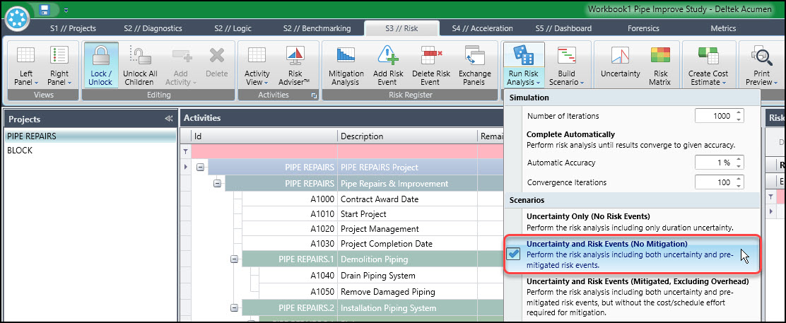 Figure 16
We click the Run Risk Analysis button; the Monte Carlo analysis runs and outputs the histogram, S-curve, and tabulated data in Figure 17.
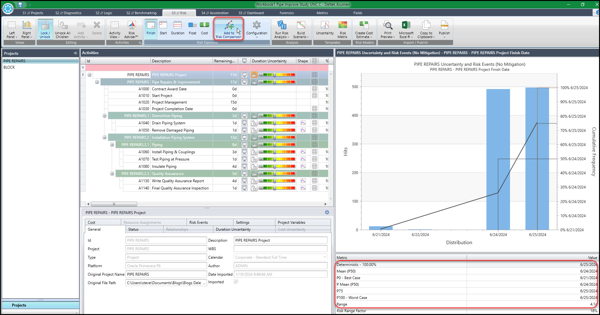 Figure 17
We click the Add to Risk Comparison button to copy the S-curve to the Risk Exposure Comparison.
Continuing, we left-click the BLOCK schedule in the navigator pane, Figure 18.
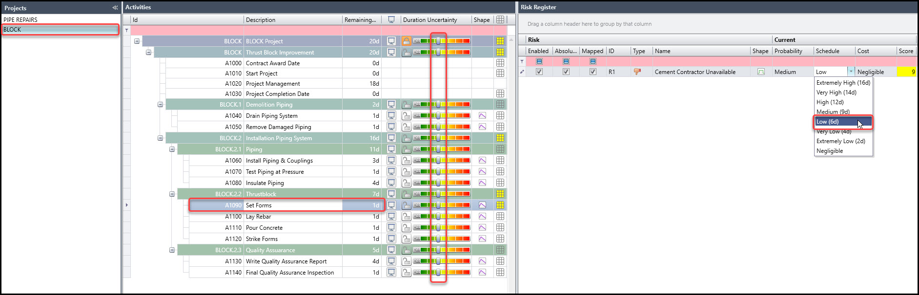 Figure 18
The duration uncertainty slider is again set to Conservative. This pipe repair and improvement project includes the risk that the thrust block installation contractor is unavailable when required. To define this risk, we create the cement contractor unavailable risk event, Figure 18.
We then map the Risk Event to the Set Forms task, Figure 18, which is the first activity in the thrust block installation process. The Risk Event probability is set to Medium (25% to 50%), and the Schedule impact is set to Low (6d).
Note in Figure 19 that when we click the risk matrix button, we previously specified Low schedule impact as six days or less.
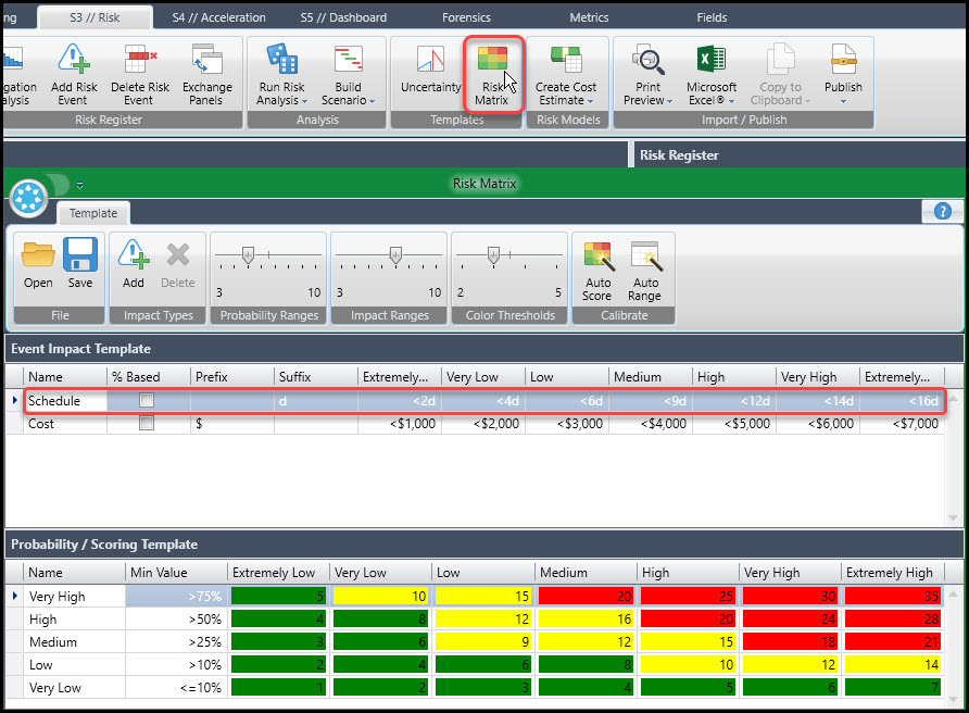 Figure 19
As before, we set the Scenario to Uncertainty and Risk Events (No Mitigation), Figure 20.
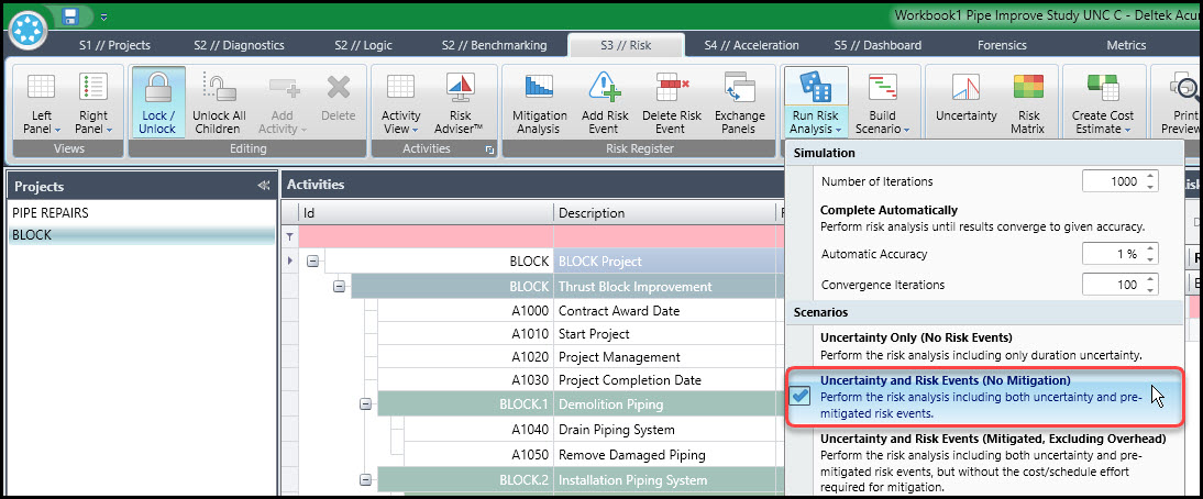 Figure 20
We click the Run Risk Analysis button. Figure 21 displays the histogram, S-curve, and tabulated output.
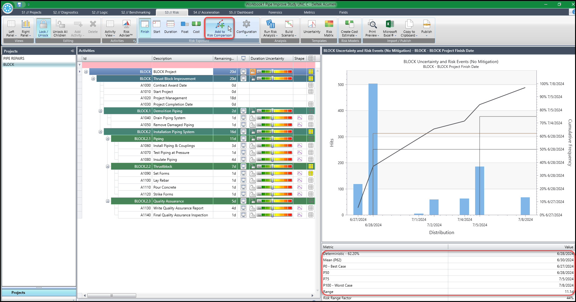 Figure 21
We click the Add to Risk Comparison button to add the S-curve to the Risk Exposure Comparison, Figure 21. We choose Right Panel | Risk Exposure Comparison, Figure 22, to display a graph of our results.
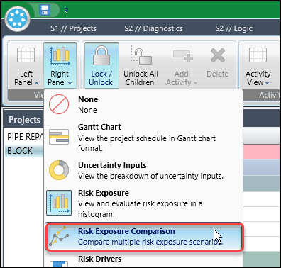 Figure 22
The Risk Exposure Comparison of the two schedules appears in Figure 23.
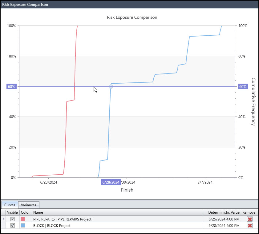 Figure 23
We click between the two S-curves at the 60% Cumulative Frequency level, Figure 23. This inserts a variance line between the two schedule plots to measure the delay from the thrust block installation. We repeat at the 80% confidence level. The resulting graph is displayed in Figure 24.
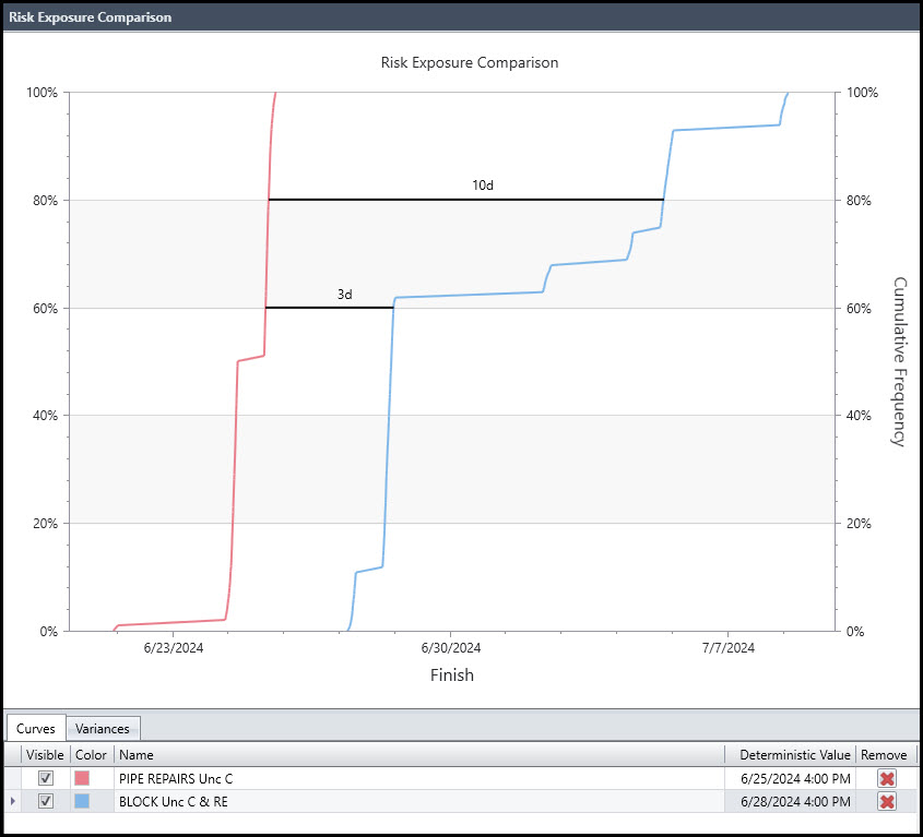 Figure 24
The first schedule result, Figure 24, is the Pipe Repairs schedule and conservative duration uncertainty. The second plot, Figure 25, is the Block schedule, including conservative duration uncertainty and a risk event.
Observe that at a 60% cumulative frequency, the additional installation of the thrust block only adds three days to the project duration. However, at an 80% certainty, the addition of the thrust block installation prolongs the schedule by ten days, which is a material delay considering the overall short duration of the project.
Note the large increase in schedule duration we must accept for the assurance or certainty above 60%.
Summary
So you can perform a multiple-schedule risk exposure comparison in Acumen Risk. We can import two schedules in Deltek Acumen and link them to the same workbook. Then, we simultaneously run schedule quality metrics diagnostics of these projects to confirm schedule health in preparation for risk modeling.
We can model uncertainty in duration estimates and risk events as required for each schedule. After risk modeling, we run a Monte Carlo analysis for each schedule for a specified number of iterations. Acumen Risk generates a histogram plot, S-curve, and tabulated data, including deterministic output.
After running each schedule analysis, we add the results to the Risk Comparison—the resulting Risk Exposure graph plots S-curve schedule outcomes and respective confidence levels. This way, we have two or more risk-adjusted schedules on a single graph, making for an efficient multiple-schedule risk exposure comparison.