Deltek Cobra supports a wide range of forecasting options, including some very flexible statistical forecasting in Cobra. However, one question is “At what point during the project lifecycle should I start running statistical forecasts?”.
At first glance this may seem like a strange question. But for anyone who has had to setup their first Earned Value Management System (EVMS), the answer is not immediately clear. In fact, even for more experienced cost analysts, knowing when to pull the trigger on statistical forecasting in Cobra can be tricky.
The reason for this is that, like so many aspects of EVM, statistical forecasting it’s both an art and a science, so you certainly can’t lay down any hard and fast rules. However, you sure can set out some guidelines. And guidelines can help you interpret the situation, in order to determine if a statistical forecast is a valuable exercise at this stage of the project’s lifecycle. And if it is a good time, what type of forecast might you consider using.
While there are entire web sites dedicated to this topic, I will be confining this article to some general guidelines with an emphasis on the capabilities of statistical forecasting in Cobra.
The Basics
Manual Forecasting vs. Statistical Forecasting in Cobra
In any EVM project, you should at the very minimum setup one manual forecast so that – at the outset of the project – you can generate an Estimate At Completion (EAC) value that is exactly equal to the Budget At Complete (BAC) value.
In Deltek Cobra, I always recommend that the analyst sets up a Manual Forecast (Retain ETC) cost class at the outset of the project. We do not need a statistical forecast at this point for a number of reasons, but the main one for “pre-go live” projects being, that you have no data upon which to trend the project, so it actually won’t do anything meaningful. I’ll get into the other reasons a bit later.
From here on out it gets a little more complex, and when you are new to EVM and/or Cobra, can be a little daunting. I recall in my early days as a Cobra Cost Analyst, being very confused about when to best perform a statistical forecast vs. a manual forecast, and what type of method to use. My goal with this article is to share what I’ve learned from some of the very best thought leaders in EVM – sage advice calmly administered to me in the midst of EVM ramp up, baselining and go live.
Statistical Forecasting Guideline #1
Do not perform statistical forecasting in Cobra during atypical phases of a project unless your intention is to verify the outcome of that particular situation.
This advice most typically refers to the ramping up period of the project. Depending on its overall duration, you may want to avoid doing any statistical forecast analysis until you have at least 3 reporting periods of progress on the books. Because projects are by definition unique efforts, the ramp up is usually anything but typical.
New teams are being formed that don’t know how to work together yet. New people with new specializations are located and hopefully hired, as well as HR, PR, Finance and Legal department onboarding processes.
On top of all this, there are always procurement delays as new equipment is purchased, premises need to be rented, sites need to be prepared, need I go on?
The point is, unless this is a project that is very similar to previous work performed by this organization, chaos is the general order of things and so projects nearly always underspend and underperform compared to baseline in the first two or three months from project go live. So, doing a statistical forecast using say, a Cum To Date CPI would only serve to quantify the insanity, with an equally insane and likely terrifying EAC. Don’t do that.
One more thought about the atypical phase might look like this. The project has been moving along nicely with a CPI staying within spitting distance of the ideal 1.0, when suddenly some high value material that has already been paid for, is still not on the loading dock, so you can’t earn any value. Your CPI tanks for the current period but your supplier assures you it will be there in 10 days, just as soon as the stuff gets released by the customs inspectors at the port.
Thus, your CPI is temporarily showing a 0.74 for the current reporting period thanks to this unexpected and very large cost variance. A statistical forecast would trend such an issue right through the project and your EAC will indicate a huge overspend at completion that simply isn’t going to be the case.
Statistical Forecasting Guideline #2
Be willing to use different statistical methods depending on current project conditions.
What does that mean? It means that choosing just one statistical forecast method and sticking with it throughout the project lifecycle, no matter what, will not always yield useful data. In fact, this approach could lead to some downright alarming EAC figures and should be avoided.
Cobra provides various statistical forecasting methods for a very good reason – what may be appropriate for one project or situation within a project, may be completely inappropriate for another.
I think this point has come about because the forecasting methods are not well understood. The Cost Analyst, for example, inherited the project and an instruction to run a certain statistical forecast every month. With the passage of time, that forecasting method may have become redundant, and the results are less than helpful to the project controls team. This goes hand-in-hand with the next guideline…
Statistical Forecasting Guideline #3
Make sure you understand the statistical forecasting methods you are using.
It seems almost a silly statement, but I have to admit that when I first started using Detlek Cobra I was hesitant to work with statistical forecast methods because I wasn’t entirely conversant with their intended purpose.
Let’s look at some examples of Cobra forecasting methods now and I’ll try and point you in the right direction.
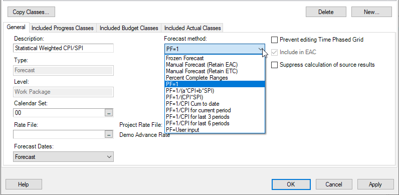
PF = 1 – Can be used at most stages of the project – assumes no trend
This is the most passive of the Cobra forecast methods and if you do want to use a prevailing statistical class, and as long as the actuals are reasonably close to expectations, this one will help retain the glass panes in the Program Managers office windows.
It basically doesn’t trend, but calculate the ETC by subtracting EV from BAC. You’ll see this expressed as PF = 1 (EV-BAC). This implies that performance is following the budget.
PF = 1/CPI Cum to date – may yield useful results after 3 – 6 reporting periods
This is the first of the methods that will trend based upon the average CPI, in this case from inception to date. I prefer to use this one only after the project is well under way, and assuming it didn’t have a very bad start. That is to say, if project ramp up was a mess, I might prefer to use this method much later in the lifecycle to give the averages time to smooth out the initial spikes.
But if the project got off to a reasonable start, this is definitely a good method to use after 3 or more reporting cycles for your statistical EAC. It is also better at absorbing spikes and dips in performance as you get further along in the lifecycle.
PF = 1/CPI current period – can be used at any time after project start, but will yield scary EACs during atypical reporting periods
I should add to the above statement that the earlier you start using this, the more apparent impact an atypical period will have on the EAC. The more periods you have ahead of you within which to calculate and apply a bad trend, the worse it can look for the final EAC. I may however, set one of these methods up in a project during an atypical period if there’s some chance that the situation causing such woe in the indices may become typical.
PF = 1/CPI last 3 periods & PF = 1/CPI last 6 periods – a good ‘go-to’ method for most situations.
I’ve put these two together because as their name suggests they are similar in function, if not in duration. These are my go-to statisticals and which of the two I choose will depend in project duration, and again where the project is in terms of percent complete.
It goes without saying that we would not have much use for either of these in the first two periods, and while I might create the cost class ready to go, wont start running these until reaching the minimum number of periods that makes sense. I like these because while their 3 or 6 month moving average smooths out some of the CPI bumps, they are still able to show an impact on the EAC, again without putting my long-suffering PM back on the anxiety meds.
PF = 1/ User Input – Used when none of the existing options would provide a fair EAC assessment
This one is not for the faint of heart. It basically allows you to run roughshod over the existing index values and enter your own decimal for ETC calculation. Like all custom options it requires you put in the time to devise a realistic number for Cobra to trend upon. How you arrive at such a number would be the subject for another article, but suffice to say if you’ve got it, Cobra can use it.
PF = 1/CPI(a*CPI) + (b*SPI) – Used when you want to weight cost and performance indices
Up to now, all our statistical forecasts have focused on just the cost performance index (CPI), but this one allows you to trend based on a weighted blend of cost and performance index values. So, if your CPI is a bit stinky, but your team are steaming well ahead of plan and spending the money faster than expected, you can show that in the EAC. Nice.
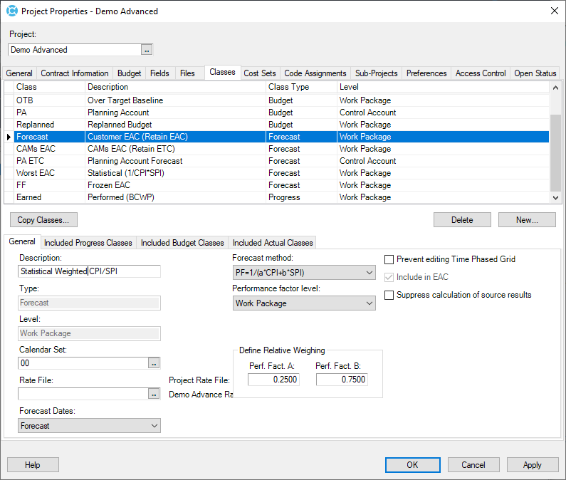
The ‘a’ and ‘b’ items referred to in the formula are user-entered variables that allow you to type in a number. So, if you wanted the SPI to have 4 times the weight than the CPI then you’d enter .25 in ‘a’ and .75 in ‘b’ and Cobra will calculate accordingly.
PF = 1/(CPI*SPI) – Used when you want to include performance as well as cost
This is rather like the previous method only you do not have the option to weight the CPI against the SPI or vice versa. Again, this could help smooth out the EAC spikes if one of your indexes are falling behind expectation.
Percent Complete Ranges – Used on long duration projects and control accounts
This is a very sophisticated feature and not for the beginner. The idea of this options is based upon something I’ve been talking about during some of the other explanations. The idea that at different times during the project lifecycle, a different statistical forecasting method may be more appropriate.
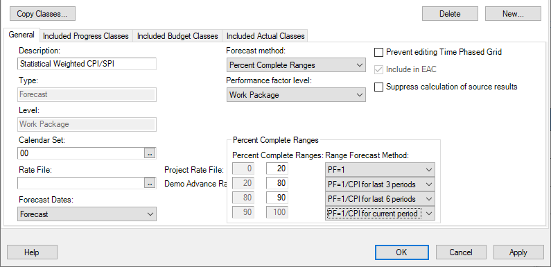
As you can see in the above example, the table allows you to select custom percent ranges, and assigned them to a different statistical method. Use of this will be optimum on longer duration projects with similarly long duration control accounts. Correctly scaled work packages may be too low a performance factor level for option, although it’s quite possible to set it up that way.
Summary
In this article, I’ve tried to alert you to the fact that forecasting is all about balancing the method you use with where your project happens to be in the lifecycle. When considering statistical forecasting in Cobra in particular, we much keep in mind that is as much a matter of when, as it is a matter of what.
We shouldn’t use a current period performance factor when the project is just starting out for example. It wouldn’t make a lot of sense to use a 6-month moving average factor, 3 periods in to a new project, and we probably don’t want to use PF = 1 when our indices have broken adrift: at least not if we’re actually interested in what they mean for our outcome.
This is not to say that we are trying to fudge the numbers or hide something, certainly not. Because this is forecast who would we be trying to kid anyway? No: what we are always trying to do is understand what our outcome might be if a particular trend continues. If our CPI is at 0.8, what is our worst, and best-case scenario? And what performance factors will tell us that?
I hope this has given you some ideas to think about. It is rather high-level I know, but it’s an interesting topic and something we should always consider carefully before committing to one statistical forecasting in Cobra method over another.